De-duplicating cells in Excel-Solution 1

While working with databases in Microsoft Excel - yes, you heard me right... Excel is perhaps the best database tool that you can START off with - it gives you the flexibility to explore while not having to deal with all the constraints placed by traditional database software. If you are about to import some data into your CRM system, it pays to have a look at the data inside Excel, just to make sure that everything looks OK before proceeding.
One of the primary functions of cleaning names is to make sure that you have filtered out the duplicate information before importing the data into your CRM system. The following tutorial will show you one of the many ways of de-duplicating data in Excel. I will cover the remaining methods in subsequent tutorials.
Summary
In this exercise we will de-duplicate a set of names provided in three columns in the format Saluation , First Name and Last Name , using the Excel's Advanced Filter option.
Detailed Solution
-
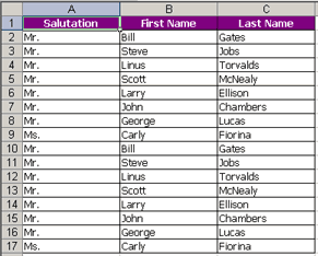
The table that we have to de-duplicate has three columns. They are Salutation, First Name and Last Name. For the purposes of this tutorial, each name has be duplicated once.

-
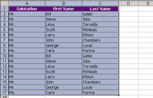
Higlight the selection from cell A1 to C17 .

-
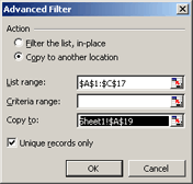
Go to Main Menu >> Data >> Filter >> Advanced Filter. Under Action , choose Copy to another location . You can also choose to Filter the list, in place , but this would mean that you will have the filtered records in the background. We have undertaken this exercise to weed out the unwanted records, so we will Copy to another location . In the Copy to field enter the cell reference of where you want the fileterd list to be copied. For this example enter Sheet1!$A$19 . Finally, select the option Unique records only . Press OK .

-
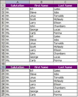
You will see the resulting table copied at below the original table.
